Inside the Power Rankings
Each component of the power rankings are explained here
LSQ
The Least Squares (LSQ) ranking is a predictive metric based on the linear-win-difference-ratio method . Generally speaking, it uses score differential and an iterative process to derive ranking scores by minimizing a chi square metric.
The goal of the rankings is to create a prediction for the result, $R_{g}$, of each game, $g$. The result should only depend on the scores of the two teams playing: $S_h$ (score, home team), and $S_a$ (score, away team). The score difference, $\Delta S_{ha}$, is used to characterize the result. To protect against anomolously large score differences, a truncated score difference is defined: $$\Delta S_{trunc} = \Delta S_{max}\text{tanh}\left(\frac{\Delta S_{ha}}{\Delta S_{max}}\right)$$ where $\Delta S_{trunc}\simeq \Delta S_{ha}$ for small values of $\Delta S_{ha}$, and $\Delta S_{trunc}\simeq \Delta S_{max}$ for large values of $\Delta S_{ha}$.
In the end, winnning a game is important with respect to making the playoffs. A win bonus, $B_w$, is added to the result, $R_g$. Finally, a score ratio is included to scale the margin of victory, and give a better indication of how close the game was: $$\frac{\Delta S_{ha}}{S_w}$$ where $S_{w}$ is the score of the winning team. This is weighted with a score ratio weight, $B_{r}$, so that the final result function is: $$R_{g}(S_{h}, S_{a} |B_{w}, \Delta S_{max}, B_{r}) = B_{w}+ \Delta S_{trunc} + B_{r}\frac{\Delta S_{ha}}{S_{w}}$$
A prediction function, $P_{g}(r_h, r_a)$, for game $g$, tries to estimate $R_g$ based on the rankings of the home team ($r_h$) and away team ($r_a$): $$P_g(r_h,r_a) = r_h - r_a = \sum_{i=1}^{i=N_t}\delta_{gt}r_t, \text{where}\ \delta_{gt} = \begin{cases} 1, & \text{if}\ t=h \\ -1, & \text{if}\ t=a\\ 0 & \text{if}\ t\neq h,a \end{cases}$$ where $P_g$ is assumed to depend linearly on the team rankings. If the season has $N_g$ games, and there are $N_t$ teams, there will be $N_g$ measurements of the $N_t$ rankings ($\vec{r}$) during the season. A chi square function is used to minimize the difference betweent he prediciton function and the result funciton: $$\chi^2(\vec{r}) = \sum_{g=1}^{N_g}\left[\frac{R_g(\vec{\alpha}) - P_g(\vec{r})}{\sigma_g} \right] = \sum_{g=1}^{N_g}\left[\frac{R_g(\vec{\alpha}) - \sum_{t=1}^{N_t}\delta_{gt}r_t}{\sigma_g} \right]$$ where $\sigma_g$ is the measurement error for each game.
A design matrix, $A_{gt}$, is identified: $$A_{gt} = \frac{\delta_{gt}}{\sigma_g}$$ A weighted result vector, $b_g$, is identified: $$b_g = \frac{R_g}{\sigma_g}$$ The ranking strength parameter, $\vec{r}$, is thus solved for using the least square minimization of the matrix equation: $$\chi^2 = |A\cdot r - b|^2$$
A game between two teams of approximately equal rank will yield a good measurement of the true ranks, so a larger weight is applied to these games. The chi square minimization is done iteratively: initially the weights, $w_g$, are set the same for each team: $$w_g^{(1)} = \frac{1}{\sigma_g^2} = 1$$ During the second iteration, the weights are set such that: $$w_g^{(2)} = \text{exp}\left(-\frac{|r_h-r_a|}{\alpha_w}\right)$$ where $\alpha_w$ is determined by: $$\text{exp}\left(-\frac{\text{max}(r_t)-\text{min}(r_t)}{\alpha_w}\right) = \frac{1}{\beta_w^2}$$ A game between the best and worst team has a measurement error $\beta_w$ times larger than when two equally ranked teams play.
2SD
The Two Step Dominace Matrix Method is based on directed graphs. A more sophisticated version is currently under consideration, much like the PageRank algorithm Google developed to rank importance of websites.
To show the basic workings of the algorithm, a walkthrough is presented for a simplified 2SD scenario: assume there are 6 teams in the league, labeled A-F. If team A beats team B, an arrow is drawn from A to B. Consider the graph below after 3 games:
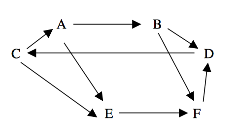
This information can be stored in a matrix where entry $d_{ij}=1$ if team $i$ beats team $j$. For this example, the matrix is: $$\begin{align}&&&\quad \text{Opposing Team} \nonumber\\ &&& \begin{matrix}A&B&C&D&E&F\end{matrix} \nonumber\\ D_{1}&=&\begin{matrix}A\\B\\C\\D\\E\\F\end{matrix} & \begin{bmatrix} 0 & 1 &0 & 0 & 1 &0 \\ 0 & 0 & 0 &1 & 0 &1 \\ 1 & 0 & 0 &0 & 1 &0 \\ 0 & 0 & 1 &0 & 0 &0 \\ 0 & 0 & 0 &0 & 0 &1 \\ 0 & 0 & 0 &1 & 0 &0 \end{bmatrix} \end{align} $$
This is called a first order dominance matrix, merely counting wins. A second order dominance matrix counts how many paths of length two exist from team $i$ to team $j$. A second order dominance over team $j$ occurs when team $i$ beats a team who beat team $j$. In the example diagram, there are two paths from A to F, so the component $d_{AF}=2$. Instead of counting lines, an easier approach is to simply square our first order dominance matrix. Continuing the example this gives: $$\begin{align}&&&\quad \text{Opposing Team} \nonumber\\ &&& \begin{matrix}A&B&C&D&E&F\end{matrix} \nonumber\\ D_{2}&=&\begin{matrix}A\\B\\C\\D\\E\\F\end{matrix} & \begin{bmatrix} 0 & 0 &0 & 1 & 0 &2 \\ 0 & 0 & 1 &1 & 0 &0 \\ 0 & 1 & 0 &0 & 1 &1 \\ 1 & 0 & 0 &0 & 1 &0 \\ 0 & 0 & 0 &1 & 0 &0 \\ 0 & 0 & 1 &0 & 0 &0 \end{bmatrix} \end{align} $$
The two step dominance method adds the first and second order dominance matrices, $\alpha_1D_1+\alpha_2D_2$, and then sums the rows in the resulting matrix. The sum represents the overall dominance score for the team corresponding to that row. Using $\alpha_1=1, \alpha_2=0.5$, our example becomes: $$\begin{align} D_{1}+0.5D_2\quad&=&\begin{matrix}A\\B\\C\\D\\E\\F\end{matrix} & \begin{bmatrix} 0 & 1 &0 & 0.5 & 1 &1 \\ 0 & 0 & 0.5 &1.5 & 0 &1 \\ 1 & 0.5 & 0 &0 & 1.5 &0.5 \\ 0.5 & 0 & 1 &0 & 0.5 &0 \\ 0 & 0 & 0 &0.5 & 0 &1 \\ 0 & 0 & 0.5 &1 & 0 &0 \end{bmatrix}\nonumber\\&&& \nonumber\\ \overset{\mbox{Sum rows}}{\longrightarrow} && \begin{matrix}A\\B\\C\\D\\E\\F\end{matrix} & \begin{bmatrix}3.5\\3\\3.5\\2\\1.5\\1.5\end{bmatrix} \nonumber \end{align} $$
In the actual rankings the weights are set to $\alpha_1=0.75$ and $\alpha_2=0.25$, and a time weighting factor is introduced, so that an entry $d^1_{ij}$ in the first order dominance matrix is: $$d^1_{ij} = 0.5 + \frac{1}{2}\left(\frac{t_g}{T}\right)$$ where $t_g$ is the time the game was played, and $T$ is the time at computing the rankings. Thus a win from the most recent week will have weight $1$, and older games tend towards $\frac{1}{2}$.
Colley
The Colley Matrix method was originally developed to rank college football teams in an unbiased, open source way. Most notably, it tries to:
- Use minimal assumptions
- Address strength of schedule
- Ignore blowouts
- Produce common sense results
The Colley Matrix only factors in wins and losses. In college football, the motivation is to combat the tendancy for teams to run up the score to improve their rankings. In fantasy football, if you're not running up the score, you're not playing the game. In that sense, the Colley rankings may be incomplete when it comes to fantasy; nevertheless, it can still offer a useful metric. Since every team plays a different schedule, factoring wins and losses should also somehow account for the quality of those wins and losses.
To begin, instead of a simple winning percentage, a rankings metric is defined by: $$\begin{equation} r = \frac{1+n_w}{2+n_{tot}}\label{eq:r} \end{equation}$$ with $n_w, n_{tot}$ designating the number of wins and total number of games respectively. This is especially important for early season rankings where winning percentages of 0% and 100% offer little comparative insight. The idea is that everyone starts with $r=\frac{1}{2}$, and with each game the ranking adjusts according to the result in a bayesian manner.
To account for strength of schedlue, the rankings metric in \eqref{eq:r} can be utilized. Consider rewriting the number of wins for team $i$ as: $$\begin{align} n_{w,i}\quad & = &\frac{n_{w,i}-n_{l,i}}{2} +\frac{n_{tot,i}}{2}\nonumber \\ & = &\frac{n_{w,i}-n_{l,i}}{2} +\sum^{n_{tot,i}}\frac{1}{2}\nonumber\\ \end{align}$$ Recognizing that the sum is the sum of the rankings of team $i$'s opponents, an effective number of wins can be defined, which accounts for strength of schedule: $$\begin{equation} n^{eff}_{w,i} \quad=\quad \frac{n_{w,i}-n_{l,i}}{2} +\sum_j^{n_{tot,i}}r_j^i \end{equation}$$
By substituting this new $n^{eff}$ into the original rankings metric in \eqref{eq:r} (and rearrange), a system of equations can be set up: $$\begin{equation}(2+n_{tot,i})r_i -\sum_{j}^{n_{tot,i}}r_j^i \quad =\quad 1 + \frac{n_{w,i}-n_{l,i}}{2} \label{eq:sys_eq}\end{equation}$$ By collecting terms, this can be written as a matrix equation: $$\begin{equation}C\vec{r}\quad=\quad\vec{b}\label{eq:mat}\end{equation}$$
In equation \eqref{eq:mat}, $\vec{b}$ is a column vector consisting of the right hand side of equation \eqref{eq:sys_eq}, and $\vec{r}$ is a column vector of all the ratings. The Colley matrix, $C$, has elements: $$c_{ii}\quad = \quad 2+n_{tot,i}\\ c_{ij}\quad=\quad -n_{ji}$$ where $n_{ji}$ is the number of times team $i$ has played team $j$. The rankings vector, $\vec{r}$, can be solved numerically rather easily since $C$ is real, symmetric and positive definite.
SOS
There are a few ways to determine strength of schedule. Colley already attempts to address this in some form, but the power rankings include an explicit metric for SOS. Since a few ranking metrics are available already, strength of schedule is calculated by weighing a team's opponent's LSQ ranking. $$\begin{equation}R_{sos}\quad=\quad \frac{1}{n_{g}}\sum_i^{n_g}\left( R_{lsq,i} \right)^{\beta_{w}} \end{equation}$$ where the exponent $\beta_w$ is chosen to give more weight to harder opponents. A value of 2.37 is chosen as it offers adequate separation between playing easier and harder opponents.
Luck
The luck index is a metric that tries to account for two common concerns:
- An opponent scoring above their average when playing you
- Outscoring teams you aren't playing
To address the first point, an average opponent performance index is calculated: $$P_{opp}\quad=\quad \frac{1}{n_g}\sum_{i}^{n_g}\frac{s_{opp,i}}{\lt{s_{opp,i}}\gt}$$ where $s_{opp,i}$ is the score of your $i^{\rm th}$ opponent, and $\lt s_{opp,i}\gt$ is your $i^{\rm th}$ opponent's average score.
To address the second point, a win index, or Windex™, is calculated for your team: $$W_{\rm index}\quad = \quad \left.\frac{n_w}{n_w+n_l}\middle/ \frac{n_{aw}}{n_{aw}+n_{al}}\right.$$ where $n_{aw}, n_{al}$ are your aggregate wins and losses. The number of aggregate wins and losses are calculated by comparing your score each week to every other team's score.
A lucky team will have $P_{opp}\lt 1$ and $W_{\rm index}\gt 1$. The Luck index weighs these two quantities: $$\begin{equation}L\quad = \quad \alpha_{P}\frac{1}{P_{opp}}+\alpha_{W}W_{\rm index}\end{equation}$$ such that a team with average luck has $L=1$, and a team with above average luck has $L\gt 1$. The power rankings try to offer a boost to teams that have been unlucky. The final luck ranking is therefore the inverse of the luck metric: $$R_{luck} = \frac{1}{L}$$ A larger value of $R_{luck}$ (small value of $L$, thus very unlucky) receives a larger boost in the rankings.
Power
Besides the 5 metrics described above, the overall power ranking also takes into account winning streaks and a consistency metric. A small winning streak bonus is added for streaks at least two games long. The consistency metric is calculated by: $$R_{cons} = s_{min}+s_{max}+s_{avg}$$ where $s_{min}, s_{max}, s_{avg}$ are a team's minimum, maximum, and average scores for the season.
Each of the component rankings are normalized so they can be weighted in a straight forward manner, and easily compared. The metrics are scaled such that the maximum rank in the league corresponds to a rank of 1.000.
The overall power ranking is thus: $$\begin{align}R_{\text{power}}\quad &=& \alpha_{lsq}R_{lsq} + \alpha_{2sd}R_{2sd} + \alpha_{colley}R_{colley} + \alpha_{sos}R_{sos} \ + \nonumber \\ && \alpha_{luck}R_{luck} + \alpha_{cons}R_{cons} + \alpha_{streak}W_{\gt2} \end{align}$$
Tier
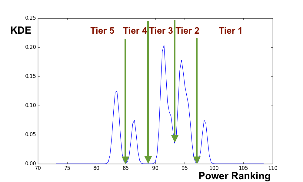
To determine the tiers, a Gaussian Kernel Density Estimation (KDE) method is used. Given a list of overall power scores, the KDE attempts to create a smooth probability density funciton. By looking for minima in the KDE, it is possible to identify separated clusters of rankings.
The KDE method is highly sensitive to the specified bandwidth: the range over which the KDE is allowed to vary. If the bandwidth is too large, there is oversmoothing, too small and each data point will be isolated. From week to week a bandwidth is selected such that it produces 3-6 tiers. An example output of the KDE method is shown below: